Collision Probability Method

Key Facts

Read this before modifying the CP solver.

• CP works with scalar flux \(\phi\), not angular flux \(\psi\)

• \(P_{ij}\) = probability that neutron born in j has first collision in i

• Convention: P[i,j] = birth in j, collision in i; flux update uses \(P^T\) (see Scattering Matrix Convention)

• Row sums = 1 (conservation), reciprocity: \(\Sigma_{t,i} V_i P(i,j) = \Sigma_{t,j} V_j P(j,i)\)

• Slab: \(E_3\) exponential-integral kernel (scipy.special.expn)

• Cylinder: \(\text{Ki}_4\) Bickley-Naylor kernel (20,000-point lookup table)

• Sphere: exponential kernel

• White-BC approximation: isotropic return at cell boundary → ~1% gap vs reflective SN

• Inner iteration IS needed: self-scatter \(\Sigma_s(g \to g) \cdot \phi_g\) makes source depend on solution

• Gotcha: tautological residual if checking denom * phi - transported (ERR-016)

• Power iteration tolerance keff_tol=1e-7 bounds eigenvalue error to ~1e-6

• Gauss-Seidel update uses latest flux immediately; Jacobi uses previous iteration

• Verification uses synthetic cross sections, not real nuclear data

Conventions

• Scattering matrix: Scattering Matrix Convention — SigS[g_from, g_to], source uses transpose

• Multi-group balance: (5) in Homogeneous Infinite-Medium Reactor

• Cross sections: Cross-Section Data Pipeline

• Verification: Cross-Section Library — regions A/B/C/D

• Eigenvalue: The Power Iteration Algorithm shared with all deterministic solvers

Overview

The collision probability (CP) method solves the multi-group eigenvalue problem in integral form. Rather than tracking the angular flux \(\psi(\mathbf{r}, \hat{\Omega}, E)\) as in discrete ordinates or method of characteristics, the CP method works directly with the scalar flux \(\phi(\mathbf{r}, E)\) by integrating out the angular variable analytically.

The key quantity is the collision probability \(P_{ij}\): the probability that a neutron born uniformly and isotropically in region \(i\) has its first collision in region \(j\) [Stamm1983]. Once the \(P_{ij}\) matrix is known, the transport problem reduces to a matrix equation in the region-averaged scalar fluxes.

Three geometries are supported:

• Slab (1D Cartesian) — the \(E_3\) exponential-integral kernel

• Concentric cylinders (1D radial) — the \(\text{Ki}_3\) / \(\text{Ki}_4\) Bickley–Naylor kernel

• Concentric spheres (1D radial) — the exponential kernel with \(y\)-weighted quadrature

All three share a single eigenvalue solver through the CPMesh augmented-geometry pattern.

Derivation sources. The analytical eigenvalues and CP matrices used for verification are computed independently by the derivation scripts. These are the source of truth for all equations in this chapter:

• derivations/cp_slab.py — slab \(E_3\) kernel via _slab_cp_matrix()

• derivations/cp_cylinder.py — cylindrical \(\text{Ki}_4\) kernel via _cylinder_cp_matrix() (uses BickleyTables)

• derivations/cp_sphere.py — spherical \(e^{-\tau}\) kernel via _sphere_cp_matrix()

• derivations/_kernels.py — \(E_3\) via e3(), \(\text{Ki}_3\)/\(\text{Ki}_4\) via BickleyTables

• derivations/_eigenvalue.py — shared eigenvalue computation via kinf_from_cp() and kinf_homogeneous()

Every equation in this chapter can be verified against these scripts. Every numerical value cited was produced by them.

Architecture: Base Geometry and Augmented Geometry

The CP solver separates geometry description from solver logic through two layers:

1. Base geometry — Mesh1D stores cell edges, material IDs, and the coordinate system. It computes volumes and surfaces via compute_volumes_1d() and compute_surfaces_1d().

2. Augmented geometry — CPMesh wraps a Mesh1D and adds the CP-specific kernel, quadrature, and CPMesh.compute_pinf_group(). The kernel is selected automatically from the mesh’s coordinate system via a match statement in CPMesh.__init__().

3. Solver — solve_cp() creates a CPMesh, builds the \(P^{\infty}\) matrices for all energy groups, and runs power iteration via CPSolver (satisfying the EigenvalueSolver protocol).

Mesh1D (edges, mat_ids, coord)
    |
    v
CPMesh (kernel + quadrature + compute_pinf_group)
    |
    v
solve_cp() -> CPResult

Design rationale (CP-20260404-001). Adding a new geometry requires only a new _setup_*() method and kernel function — the eigenvalue solver, post-processing, and plotting are geometry-agnostic. The alternative (three separate solver classes) would duplicate ~200 lines of iteration logic. The derivation modules mirror this: all three _*_cp_matrix functions have identical white-BC closure code, differing only in the kernel and quadrature.

The Integral Transport Equation

Starting point: the steady-state, one-speed transport equation in integral form. For a neutron born at \(\mathbf{r}'\) travelling toward \(\mathbf{r}\), the uncollided flux is

(1)\[\phi^{\text{unc}}(\mathbf{r}) = \int_{V} \frac{e^{-\tau(\mathbf{r}', \mathbf{r})}}{4\pi |\mathbf{r} - \mathbf{r}'|^2} \, Q(\mathbf{r}') \, dV'\]

where \(Q(\mathbf{r}')\) is the total source (fission + scattering + external) and \(\tau(\mathbf{r}', \mathbf{r})\) is the optical path (number of mean free paths) between the two points:

(2)\[\tau(\mathbf{r}', \mathbf{r}) = \int_0^{|\mathbf{r} - \mathbf{r}'|} \Sigt{}\bigl(\mathbf{r}' + s\,\hat{\Omega}\bigr) \, ds\]

Flat-Source Approximation

The CP method assumes the source is spatially flat within each sub-region \(i\). The MOC solver uses the same approximation; see Flat-Source Approximation.

(3)\[Q(\mathbf{r}) = Q_i \quad \text{for } \mathbf{r} \in V_i\]

Under this approximation, the collision rate in region \(j\) due to sources in region \(i\) can be written as

(4)\[\Sigt{j} \, \phi_j \, V_j = \sum_i P_{ji} \, V_i \, Q_i\]

where \(P_{ji}\) is the collision probability and \(V_i\) is the volume of region \(i\).

Note

Convention: in this codebase, \(P_{ij}\) is indexed as \(P[\text{birth}_i, \text{collision}_j]\). The flux update uses \(P^T\): phi = P_inf.T @ source. This is implemented in CPSolver.solve_fixed_source(). See Why PT Appears in the Flux Update for the full derivation.

Definition of Collision Probabilities

Within-Cell Probabilities and Complementarity

For a cell with \(N\) sub-regions, the within-cell collision probability \(P_{ij}^{\text{cell}}\) is the probability of first collision in \(j\) without leaving the cell. Complementarity:

(5)\[\sum_{j=1}^{N} P_{ij}^{\text{cell}} + P_{i,\text{out}} = 1\]

where \(P_{i,\text{out}}\) is the escape probability. In the code: P_out = 1 - P_cell.sum(axis=1) (CPMesh._apply_white_bc()). Verified by test_cp_properties.py::test_row_sums for all three coordinate systems.

Reciprocity

From detailed balance [Hebert2009] section 3.2:

(6)\[\Sigt{i} \, V_i \, P_{ij}^{\text{cell}} = \Sigt{j} \, V_j \, P_{ji}^{\text{cell}}\]

Why reciprocity holds. Time-reversal invariance: a neutron born in \(i\) colliding in \(j\) traces a path identical (in reverse) to one born in \(j\) colliding in \(i\). The optical thickness along any chord is direction-independent. The factor \(\Sigt{i} V_i\) converts from “per neutron born” (probability) to “per unit source intensity” (rate), accounting for different source strengths in regions of different sizes and cross sections.

Practical consequence. The CP matrix need only be computed for \(j \ge i\); the lower triangle follows from:

\[P_{ji}^{\text{cell}} = P_{ij}^{\text{cell}} \cdot \frac{\Sigt{i} \, V_i}{\Sigt{j} \, V_j}\]

This halves the computation cost. In the code, CPMesh._normalize_rcp() divides the reduced collision probability by \(\Sigt{i} V_i\) for each row. Reciprocity is verified by test_cp_properties.py::test_reciprocity and extended to multi-group by test_cp_verification.py::TestMultiGroupProperties::test_reciprocity_multigroup.

Escape and Re-entry (White Boundary Condition)

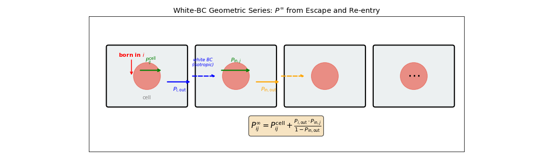
For an infinite lattice, a neutron escaping one cell immediately enters an identical neighbour. The white boundary condition assumes the re-entering angular distribution is isotropic — i.e., the neutron forgets its direction upon re-entry.

The surface-to-region probability is:

(7)\[P_{\text{in},j} = \frac{\Sigt{j} \, V_j \, P_{j,\text{out}}}{S}\]

where \(S\) is the cell surface area, accessed uniformly via mesh.surfaces[-1] (compute_surfaces_1d()):

Coordinate system	Surface area \(S\)
Cartesian (slab)	\(1\) (per unit transverse area)
Cylindrical	\(2\pi R_{\text{cell}}\)
Spherical	\(4\pi R_{\text{cell}}^2\)

Derivation of \(P_{\text{in},j}\). By reciprocity between the surface source and the volume source in region \(j\):

(8)\[\frac{S}{4} \cdot P_{\text{in},j} = \Sigt{j} \, V_j \cdot P_{j,\text{out}}\]

The factor \(S/4\) is the effective surface source strength for an isotropic inward flux on a convex surface. It originates from the Cauchy–Dirac mean chord length theorem: \(\bar{\ell} = 4V/S\) for a convex body ([Hebert2009] section 3.3). Physically: an isotropic flux crossing a convex surface sees, on average, a path length of \(4V/S\) through the interior. Solving (8):

\[P_{\text{in},j} = \frac{4 \Sigt{j} V_j P_{j,\text{out}}}{S}\]

In the standard CP formulation [Stamm1983] section 3.5, the surface-to-region probability is defined per unit inward current \(J^-\), and the normalisation convention absorbs the factor of 4. ORPHEUS uses this convention, so CPMesh._apply_white_bc() computes:

# White-BC closure (geometry-agnostic)
P_in = sig_t * V * P_out / S_cell

The surface-to-surface probability is:

(9)\[P_{\text{in,out}} = 1 - \sum_j P_{\text{in},j}\]

The same formula appears in all three derivation scripts (e.g., derivations/cp_slab.py, line P_in = sig_t_g * t_arr * P_out with the slab convention \(S = 1\), \(V = t\); and derivations/cp_cylinder.py, line S_cell = 2.0 * np.pi * r_cell with cylindrical \(V = \pi(R_k^2 - R_{k-1}^2)\)).

Infinite-Lattice CP Matrix

The infinite-lattice CP accounts for neutrons that escape, re-enter, possibly escape again (geometric series):

(10)\[P_{ij}^{\infty} = P_{ij}^{\text{cell}} + \frac{P_{i,\text{out}} \, P_{\text{in},j}} {1 - P_{\text{in,out}}}\]

This formula is identical for all three geometries when expressed in terms of \(V_i\) and \(S\). It is implemented in CPMesh._apply_white_bc() (solver) and independently in all three derivation scripts (e.g., derivations/cp_slab.py: P_inf_g[:,:,g] = P_cell + np.outer(P_out, P_in) / (1.0 - P_inout)).

import numpy as np
import matplotlib.pyplot as plt
import matplotlib.patches as mpatches

fig, ax = plt.subplots(figsize=(14, 4))

cell_w = 2.0
cell_h = 1.5
gap = 0.3
n_cells = 4

for c in range(n_cells):
    x0 = c * (cell_w + gap)
    rect = mpatches.FancyBboxPatch(
        (x0, 0), cell_w, cell_h, boxstyle="round,pad=0.05",
        facecolor='#ecf0f1', edgecolor='black', linewidth=2)
    ax.add_patch(rect)

    fuel = plt.Circle((x0 + cell_w / 2, cell_h / 2), 0.35,
                      color='#e74c3c', alpha=0.6)
    ax.add_patch(fuel)

    if c == 0:
        ax.text(x0 + cell_w / 2, 0.15, 'cell', fontsize=9,
                ha='center', color='gray')

arrow_y = cell_h / 2
ax.annotate(r'born in $i$', xy=(0.6, arrow_y), fontsize=10,
            ha='center', color='red', fontweight='bold',
            xytext=(0.6, arrow_y + 0.5),
            arrowprops=dict(arrowstyle='->', color='red', lw=1.5))

ax.annotate('', xy=(1.4, arrow_y + 0.15),
            xytext=(0.8, arrow_y + 0.15),
            arrowprops=dict(arrowstyle='->', color='green', lw=2))
ax.text(1.1, arrow_y + 0.35, r'$P_{ij}^{\mathrm{cell}}$',
        fontsize=10, ha='center', color='green')

ax.annotate('', xy=(cell_w + gap / 2, arrow_y - 0.15),
            xytext=(1.5, arrow_y - 0.15),
            arrowprops=dict(arrowstyle='->', color='blue', lw=2))
ax.text(1.85, arrow_y - 0.4, r'$P_{i,\mathrm{out}}$',
        fontsize=10, ha='center', color='blue')

x1 = cell_w + gap
ax.annotate('', xy=(x1 + 0.5, arrow_y),
            xytext=(x1 - gap / 2, arrow_y),
            arrowprops=dict(arrowstyle='->', color='blue', lw=2,
                            linestyle='dashed'))
ax.text(x1 + 0.15, arrow_y + 0.25, 'white BC\n(isotropic)',
        fontsize=8, ha='center', color='blue', style='italic')

ax.annotate('', xy=(x1 + 1.4, arrow_y + 0.15),
            xytext=(x1 + 0.6, arrow_y + 0.15),
            arrowprops=dict(arrowstyle='->', color='green', lw=2))
ax.text(x1 + 1.0, arrow_y + 0.35, r'$P_{\mathrm{in},j}$',
        fontsize=10, ha='center', color='green')

ax.annotate('', xy=(2 * (cell_w + gap) - gap / 2, arrow_y - 0.15),
            xytext=(x1 + 1.5, arrow_y - 0.15),
            arrowprops=dict(arrowstyle='->', color='orange', lw=2))
ax.text(x1 + 1.85, arrow_y - 0.4, r'$P_{\mathrm{in,out}}$',
        fontsize=10, ha='center', color='orange')

x2 = 2 * (cell_w + gap)
ax.annotate('', xy=(x2 + 0.5, arrow_y),
            xytext=(x2 - gap / 2, arrow_y),
            arrowprops=dict(arrowstyle='->', color='orange', lw=2,
                            linestyle='dashed'))

x3 = 3 * (cell_w + gap)
ax.text(x3 + cell_w / 2, cell_h / 2, r'$\cdots$',
        fontsize=24, ha='center', va='center')

ax.text(
    n_cells * (cell_w + gap) / 2, -0.6,
    r'$P_{ij}^{\infty} = P_{ij}^{\mathrm{cell}}'
    r' + \frac{P_{i,\mathrm{out}} \cdot P_{\mathrm{in},j}}'
    r'{1 - P_{\mathrm{in,out}}}$',
    fontsize=14, ha='center',
    bbox=dict(boxstyle='round', facecolor='wheat', alpha=0.8))

ax.set_xlim(-0.5, n_cells * (cell_w + gap))
ax.set_ylim(-1.2, cell_h + 0.8)
ax.set_aspect('equal')
ax.set_xticks([])
ax.set_yticks([])
ax.set_title(
    r'White-BC Geometric Series: $P^{\infty}$ from Escape and Re-entry',
    fontsize=13)
plt.tight_layout()

(png)

White-BC geometric series: a neutron born in region \(i\) either collides within the cell (\(P_{ij}^{\text{cell}}\)) or escapes, re-enters isotropically, and the chain repeats. The infinite sum converges to \(P_{ij}^{\infty}\).

Derivation of the geometric series. A neutron born in \(i\):

• Collides in \(j\) on the first pass: probability \(P_{ij}^{\text{cell}}\).

• Escapes: probability \(P_{i,\text{out}}\).

• After escaping, re-enters isotropically and collides in \(j\): probability \(P_{\text{in},j}\).

• Or traverses without collision: probability \(P_{\text{in,out}}\).

• Each subsequent escape-and-re-entry multiplies by \(P_{\text{in,out}}\).

Summing:

\[\begin{split}P_{ij}^{\infty} &= P_{ij}^{\text{cell}} + P_{i,\text{out}} P_{\text{in},j} (1 + P_{\text{in,out}} + P_{\text{in,out}}^2 + \cdots) \\ &= P_{ij}^{\text{cell}} + \frac{P_{i,\text{out}} P_{\text{in},j}}{1 - P_{\text{in,out}}}\end{split}\]

The series converges because \(P_{\text{in,out}} < 1\) (some fraction of re-entering neutrons must eventually collide).

Row sum property: \(\sum_j P_{ij}^{\infty} = 1\). Proof: substitute complementarity (5) for both sums:

\[\begin{split}\sum_j P_{ij}^{\infty} &= \sum_j P_{ij}^{\text{cell}} + P_{i,\text{out}} \frac{\sum_j P_{\text{in},j}}{1 - P_{\text{in,out}}} \\ &= (1 - P_{i,\text{out}}) + P_{i,\text{out}} \frac{1 - P_{\text{in,out}}}{1 - P_{\text{in,out}}} = 1\end{split}\]

Verified numerically by test_cp_properties.py::test_row_sums.

Warning

The white BC is an approximation. The true angular distribution at a cell boundary is anisotropic — neutrons preferentially stream in the direction of the flux gradient. The white BC smears this anisotropy into an isotropic re-entry, which overestimates the flux in optically thin regions and underestimates it in thick ones. For the 1G slab benchmark, the CP method (white BC) gives \(\keff \approx 1.272\) while SN (reflective BC) gives \(\approx 1.261\) — a ~1% discrepancy entirely due to the white-BC approximation. See Numerical Evidence: White-BC Approximation Quality.

The Three CP Kernels

The CP method requires a geometry-specific kernel function \(F(\tau)\) that encodes the angular averaging. The kernel arises from integrating the point-to-point transmission \(e^{-\tau}\) over the angular degrees of freedom eliminated by the geometry’s symmetry. The number of remaining angular integrations determines which special function appears:

Geometry	Kernel \(F(\tau)\)	\(F(0)\)	Residual quadrature
Slab	\(E_3(\tau) = \int_0^1 \mu \, e^{-\tau/\mu} \, d\mu\)	\(1/2\)	None (analytical)
Cylinder	\(\text{Ki}_4(\tau) = \int_\tau^\infty \text{Ki}_3(t)\,dt\)	\(\approx 0.4244\)	\(y\)-quadrature over chord heights
Sphere	\(e^{-\tau}\)	\(1\)	\(y\)-quadrature (\(y\)-weighted)

In all cases, the reduced collision probability is built from a second-difference of the kernel (13). This common structure is why all three geometries are handled by a single CPMesh class.

import numpy as np
import matplotlib.pyplot as plt
from scipy.special import expn
from scipy.integrate import quad

x = np.linspace(0.001, 6, 500)

e3 = expn(3, x)

ki3 = np.array([
    quad(lambda t, xx=xx: np.exp(-xx / np.sin(t)) * np.sin(t),
         0, np.pi / 2)[0]
    for xx in x
])

dx = x[1] - x[0]
ki4 = np.cumsum(ki3[::-1])[::-1] * dx

exp_kernel = np.exp(-x)

fig, ax = plt.subplots(figsize=(10, 6))
ax.semilogy(x, e3, '-r', linewidth=2, label=r'$E_3(\tau)$ (slab)')
ax.semilogy(x, ki3, '-g', linewidth=2,
            label=r'$\mathrm{Ki}_3(\tau)$ (cylinder, integrand)')
ax.semilogy(x, ki4, '--g', linewidth=2,
            label=r'$\mathrm{Ki}_4(\tau)$ (cylinder, kernel)')
ax.semilogy(x, exp_kernel, '-b', linewidth=2,
            label=r'$e^{-\tau}$ (sphere)')

ax.axhline(0.5, color='red', linestyle=':', alpha=0.5)
ax.text(5.5, 0.55, r'$E_3(0)=\frac{1}{2}$', fontsize=10, color='red')
ax.axhline(1.0, color='blue', linestyle=':', alpha=0.5)
ax.text(5.5, 1.1, r'$e^0 = 1$', fontsize=10, color='blue')

ax.set_xlabel(r'Optical thickness $\tau$', fontsize=12)
ax.set_ylabel(r'$F(\tau)$', fontsize=12)
ax.set_title('CP Kernel Functions by Geometry')
ax.legend(fontsize=11, loc='lower left')
ax.set_ylim(1e-4, 2)
ax.grid(True, alpha=0.3)
plt.tight_layout()

(png)

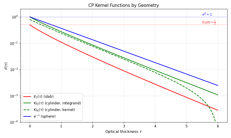
The three CP kernel functions: \(E_3\) (slab), \(\text{Ki}_3\) / \(\text{Ki}_4\) (cylinder), and \(e^{-\tau}\) (sphere). All decay exponentially; they differ in \(F(0)\) and rate of decay.

Derivation source: The kernels are implemented in derivations/_kernels.py: e3() and e3_vec() for slab; BickleyTables (with ki3_vec() and ki4_vec()) for cylinder.

Why the Kernel Differs by Geometry

Slab (1D): A neutron in a slab travels at angle \(\theta\) to the normal. The optical path scales as \(\tau / \mu\) where \(\mu = \cos\theta\). The angular flux contribution includes a factor \(\mu\) (projected area \(dA = \mu\,dA_\perp\)). Averaging the transmission \(e^{-\tau/\mu}\) over the forward half-space \(\mu \in [0, 1]\):

(11)\[E_3(\tau) = \int_0^1 \mu \, e^{-\tau/\mu} \, d\mu\]

This is one angular integration, leaving a function of \(\tau\) only. \(E_3(0) = 1/2\) and \(E_3(\tau) \to 0\) exponentially. Computed analytically via scipy.special.expn() (wrapped as _e3() in the solver and e3() in the derivations).

Cylinder (2D): The neutron travels at polar angle \(\theta\) to the cylinder axis and crosses the annular section at impact parameter \(y\). The chord length depends on \(y\) (geometry) and the optical path depends on \(\theta\) (as \(\tau / \sin\theta\)). Integrating over the polar angle yields the Bickley–Naylor function:

(12)\[\text{Ki}_3(\tau) = \int_0^{\pi/2} e^{-\tau / \sin\theta} \sin\theta \, d\theta\]

The \(\sin\theta\) weight arises from the solid-angle measure in cylindrical coordinates: \(d\Omega = \sin\theta\,d\theta\,d\varphi\). The azimuthal angle \(\varphi\) integrates trivially by symmetry; the projected ray length onto the cross-sectional plane is proportional to \(\sin\theta\); and the probability of a ray at angle \(\theta\) is proportional to \(\sin\theta\) from the \(d\Omega\) measure.

This eliminates one angular dimension, but the \(y\)-integration over chord heights remains as numerical quadrature — the second angular dimension that cylindrical symmetry does NOT eliminate.

The antiderivative \(\text{Ki}_4(\tau) = \int_\tau^\infty \text{Ki}_3(t)\,dt\) appears in the second-difference formula because the derivation involves double antiderivatives of the point-to-point kernel (see The Second-Difference Formula: Full Derivation). Why Ki₄ not Ki₃: the slab uses \(E_3\) (double antiderivative of the point kernel \(E_1\)); the cylinder uses \(\text{Ki}_4\) (single antiderivative of \(\text{Ki}_3\), which is already one integration up from the raw transmission). The second-difference formula cancels one antiderivative level, leaving \(\text{Ki}_4\).

The Ki₃ function plays the same role for cylindrical geometry that \(E_3\) plays for slab geometry: it represents the probability of a neutron travelling a certain optical distance in the medium [Carlvik1966].

\(\text{Ki}_3(0) = 1\) and \(\text{Ki}_3(x) \to 0\) exponentially. \(\text{Ki}_3\) and \(\text{Ki}_4\) are tabulated numerically by _build_ki_tables() (solver) and BickleyTables (derivations) because no closed-form expression exists. See Ki3/Ki4 Table Construction.

Sphere (3D): Full spherical symmetry absorbs all angular variables into the \(y\)-quadrature weight. The kernel is simply \(F(\tau) = e^{-\tau}\) — no special functions needed. The extra factor of \(y\) in the quadrature weight comes from the spherical area element \(2\pi y\,dy\) (ring of sources) versus the cylindrical \(2\,dy\) (line of sources). In CPMesh._setup_spherical():

# Spherical weight: extra factor of y in the quadrature
self._y_wts = self._y_wts * self._y_pts

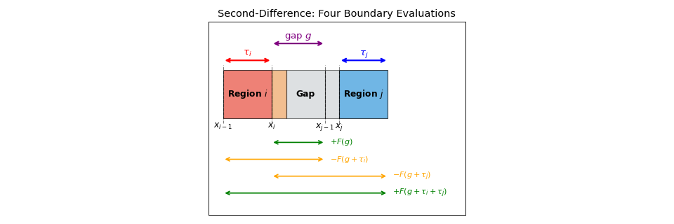
The Second-Difference Formula: Full Derivation

The reduced collision probability uses the four-term second-difference:

(13)\[\Delta_2[F](\tau_i, \tau_j, g) = F(g) - F(g + \tau_i) - F(g + \tau_j) + F(g + \tau_i + \tau_j)\]

where \(g\) is the optical gap, \(\tau_i\) and \(\tau_j\) are the optical thicknesses of the source and target regions.

Setup. Regions \(i\) and \(j\) separated by optical gap \(g\). A neutron born at optical depth \(s\) within region \(i\) (\(0 \le s \le \tau_i\)) must traverse \(d = (\tau_i - s) + g + t\) to reach depth \(t\) in region \(j\) (\(0 \le t \le \tau_j\)).

Step 1: Source-position average. Integrate the kernel over the birth position \(s\) within region \(i\). Substituting \(u = (\tau_i - s) + g + t\) (so \(du = -ds\)):

\[\begin{split}I(t) &= \int_0^{\tau_i} F\bigl((\tau_i - s) + g + t\bigr) \, ds \\ &= \int_{g+t}^{\tau_i + g + t} F(u) \, du \\ &= \hat{F}(\tau_i + g + t) - \hat{F}(g + t)\end{split}\]

where \(\hat{F}(x) = \int_0^x F(u)\,du\) is the antiderivative.

Step 2: Collision-position average. Integrate over the collision position \(t\) within region \(j\):

\[\begin{split}\text{rcp}_{ij} &= \int_0^{\tau_j} I(t) \, dt \\ &= \int_0^{\tau_j} \bigl[\hat{F}(\tau_i + g + t) - \hat{F}(g + t)\bigr] dt\end{split}\]

Evaluating each integral using the double antiderivative \(\hat{\hat{F}}(x) = \int_0^x \hat{F}(u)\,du\):

\[\begin{split}\int_0^{\tau_j} \hat{F}(g + t) \, dt &= \hat{\hat{F}}(g + \tau_j) - \hat{\hat{F}}(g) \\ \int_0^{\tau_j} \hat{F}(\tau_i + g + t) \, dt &= \hat{\hat{F}}(\tau_i + g + \tau_j) - \hat{\hat{F}}(\tau_i + g)\end{split}\]

Combining:

(14)\[\text{rcp}_{ij} = \hat{\hat{F}}(g) - \hat{\hat{F}}(g + \tau_i) - \hat{\hat{F}}(g + \tau_j) + \hat{\hat{F}}(g + \tau_i + \tau_j)\]

Step 3: Identify \(\hat{\hat{F}}\) per geometry.

Geometry	Point-to-point kernel	1st antiderivative	\(\hat{\hat{F}}\)
Slab	\(E_1(\tau)\)	\(-E_2(\tau)\)	\(E_3(\tau)\)
Cylinder	\(\text{Ki}_3(\tau)\)	\(-\text{Ki}_4(\tau)\)	\(\text{Ki}_5(\tau)\)
Sphere	\(e^{-\tau}\)	\(-e^{-\tau}\)	\(e^{-\tau}\)

For the slab, the \(E_n\) functions satisfy \(E_n'(\tau) = -E_{n-1}(\tau)\). The code evaluates (13) directly with \(F = E_3\) (slab), \(F = \text{Ki}_4\) (cylinder), or \(F = e^{-\tau}\) (sphere).

Derivation source: This four-term structure appears in all three derivation scripts. For example, in derivations/cp_slab.py:

dd = (e3(gap_d) - e3(gap_d + tau_i)
      - e3(gap_d + tau_j) + e3(gap_d + tau_i + tau_j))

And in derivations/cp_cylinder.py:

dd = (tables.ki4_vec(gap_d) - tables.ki4_vec(gap_d + tau_i)
      - tables.ki4_vec(gap_d + tau_j)
      + tables.ki4_vec(gap_d + tau_i + tau_j))

And in derivations/cp_sphere.py:

dd = (kernel(gap_d) - kernel(gap_d + tau_i)
      - kernel(gap_d + tau_j) + kernel(gap_d + tau_i + tau_j))

where kernel = lambda tau: np.exp(-tau).

import numpy as np
import matplotlib.pyplot as plt
import matplotlib.patches as mpatches

fig, ax = plt.subplots(figsize=(12, 4))

colors = ['#e74c3c', '#e67e22', '#bdc3c7', '#bdc3c7', '#3498db']
labels = ['Region $i$', '', 'Gap', '', 'Region $j$']
widths = [1.0, 0.3, 0.8, 0.3, 1.0]
positions = np.cumsum([0] + widths)

for k in range(5):
    rect = mpatches.FancyBboxPatch(
        (positions[k], 0), widths[k], 1.0,
        boxstyle="square,pad=0",
        facecolor=colors[k], edgecolor='black',
        alpha=0.5 if k in [1, 2, 3] else 0.7)
    ax.add_patch(rect)
    if labels[k]:
        ax.text(positions[k] + widths[k] / 2, 0.5, labels[k],
                ha='center', va='center', fontsize=11,
                fontweight='bold')

bnd_labels = [
    (positions[0], r'$x_{i-1}$'),
    (positions[1], r'$x_i$'),
    (positions[3], r'$x_{j-1}$'),
    (positions[4], r'$x_j$'),
]
for xp, label in bnd_labels:
    ax.plot([xp, xp], [-0.1, 1.1], 'k--', linewidth=1, alpha=0.5)
    ax.text(xp, -0.2, label, ha='center', fontsize=11)

ax.annotate('', xy=(positions[1], 1.2), xytext=(positions[0], 1.2),
            arrowprops=dict(arrowstyle='<->', color='red', lw=2))
ax.text((positions[0] + positions[1]) / 2, 1.3, r'$\tau_i$',
        ha='center', fontsize=12, color='red')

ax.annotate('', xy=(positions[4] + widths[4], 1.2),
            xytext=(positions[3] + widths[3], 1.2),
            arrowprops=dict(arrowstyle='<->', color='blue', lw=2))
ax.text((positions[3] + widths[3] + positions[4] + widths[4]) / 2, 1.3,
        r'$\tau_j$', ha='center', fontsize=12, color='blue')

ax.annotate('', xy=(positions[3], 1.55), xytext=(positions[1], 1.55),
            arrowprops=dict(arrowstyle='<->', color='purple', lw=2))
ax.text((positions[1] + positions[3]) / 2, 1.65,
        r'gap $g$', ha='center', fontsize=12, color='purple')

y_bot = -0.5
terms = [
    (positions[1], positions[3], r'$+F(g)$', 'green'),
    (positions[0], positions[3], r'$-F(g+\tau_i)$', 'orange'),
    (positions[1], positions[4] + widths[4], r'$-F(g+\tau_j)$', 'orange'),
    (positions[0], positions[4] + widths[4],
     r'$+F(g+\tau_i+\tau_j)$', 'green'),
]
for k, (x1, x2, label, color) in enumerate(terms):
    y = y_bot - k * 0.35
    ax.annotate('', xy=(x2, y), xytext=(x1, y),
                arrowprops=dict(arrowstyle='<->', color=color,
                                lw=1.5))
    ax.text(x2 + 0.1, y, label, fontsize=10, va='center',
            color=color)

ax.set_xlim(-0.3, 5.0)
ax.set_ylim(-2.0, 2.0)
ax.set_aspect('equal')
ax.set_yticks([])
ax.set_xticks([])
ax.set_title('Second-Difference: Four Boundary Evaluations',
             fontsize=13)
plt.tight_layout()

(png)

Geometric meaning of the four second-difference terms \(\Delta_2[F](\tau_i, \tau_j, g)\). Green arrows mark the two positive terms \(+F(g)\) and \(+F(g+\tau_i+\tau_j)\); orange arrows mark the two negative terms.

The Discretised Second-Difference

The continuous formula (14) is discretised by evaluating the double antiderivative at region boundary positions. Define:

(15)\[S(i, j, g) = \int_0^{R_i} \bigl[\text{Ki}_3(\tau_p(y)) - \text{Ki}_3(\tau_m(y))\bigr] \, dy\]

The within-cell collision probability for \(j \ge i\) is:

(16)\[P_{ij}^{\text{cell}} = \frac{2}{\Sigt{i} V_i} \Bigl[ S(i,j) - S(i{-}1,j) - S(i,j{-}1) + S(i{-}1,j{-}1) \Bigr] + \delta_{ij}\]

where \(\delta_{ij}\) accounts for self-collision and terms with index 0 vanish (no region interior to region 1).

Correspondence: continuous vs discrete

Continuous term	Discrete boundary evaluation
\(\hat{\hat{F}}(g)\)	\(S(i{-}1, j{-}1)\) — both inner boundaries
\(\hat{\hat{F}}(g + \tau_i)\)	\(S(i, j{-}1)\) — outer of source, inner of target
\(\hat{\hat{F}}(g + \tau_j)\)	\(S(i{-}1, j)\) — inner of source, outer of target
\(\hat{\hat{F}}(g + \tau_i + \tau_j)\)	\(S(i, j)\) — both outer boundaries

Implementation. ORPHEUS does not pre-compute the \(S\) array. Instead, CPMesh._compute_radial_rcp() evaluates the second-difference at each \(y\)-quadrature point and integrates numerically. This avoids storing \(S\) and allows the same code path for all three geometries by parameterising the kernel function. The derivation scripts use the same approach.

Self-Collision: Full Derivation

The self-collision term (\(i = j\)) cannot use the gap formula because source and collision positions overlap. The double integral is:

(17)\[r_{ii} = \int_0^{\tau_i} \int_0^{\tau_i} F_1(|s - t|) \, dt \, ds\]

where \(F_1\) is the point-to-point kernel.

Evaluation (slab case, :math:`F_1 = E_1`). Split at \(s = t\) and use symmetry (\(s > t\) half = \(s < t\) half):

\[r_{ii} &= 2 \int_0^{\tau_i} \int_0^s E_1(s - t) \, dt \, ds\]

Evaluate the inner integral using \(\int E_1(x) dx = -E_2(x)\):

\[\int_0^s E_1(s - t) \, dt &= \bigl[-E_2(s - t)\bigr]_{t=0}^{t=s} = -E_2(0) + E_2(s) = E_2(s) - E_2(0)\]

Since \(E_2(0) = 1\), the inner integral is \(E_2(s) - 1\). The outer integral:

\[\begin{split}r_{ii} &= 2 \int_0^{\tau_i} \bigl[E_2(s) - 1\bigr] ds \\ &= 2 \bigl[-E_3(s)\bigr]_0^{\tau_i} - 2\tau_i \\ &= 2 \bigl[-E_3(\tau_i) + E_3(0)\bigr] - 2\tau_i \\ &= 2 E_3(0) - 2 E_3(\tau_i) - 2\tau_i\end{split}\]

Wait — let me redo this carefully. \(\int_0^s E_1(s-t) dt\): substituting \(u = s - t\), \(du = -dt\):

\[\int_0^s E_1(u) du = \bigl[-E_2(u)\bigr]_0^s = -E_2(s) + E_2(0)\]

So the inner integral is \(E_2(0) - E_2(s)\). Continuing:

\[\begin{split}r_{ii} &= 2 \int_0^{\tau_i} \bigl[E_2(0) - E_2(s)\bigr] ds \\ &= 2 \bigl[\tau_i E_2(0) + E_3(\tau_i) - E_3(0)\bigr]\end{split}\]

Using \(E_2(0) = 1\) and \(E_3(0) = 1/2\):

\[r_{ii} = 2\tau_i + 2 E_3(\tau_i) - 1\]

The normalised self-collision probability is \(P_{ii} = r_{ii} / (\Sigt{i} t_i)\). Since \(\tau_i = \Sigt{i} t_i\):

\[P_{ii} = \frac{2\tau_i + 2 E_3(\tau_i) - 1}{\tau_i} = 2 + \frac{2 E_3(\tau_i) - 1}{\tau_i} = 1 + \frac{2 E_3(\tau_i) - 2 E_3(0)}{\tau_i}\]

which is equivalently written as:

\[P_{ii} = 1 - \frac{2(E_3(0) - E_3(\tau_i))}{\tau_i}\]

For thick regions (\(\tau_i \to \infty\)): \(E_3(\tau_i) \to 0\), so \(P_{ii} \to 1 - 1/\tau_i \to 1\). For thin regions (\(\tau_i \to 0\)): \(E_3(\tau_i) \to E_3(0) = 1/2\), so \(P_{ii} \to 0\). Tested by test_cp_verification.py::TestOpticalLimits.

In the solver code (CPMesh._compute_slab_rcp()):

# Self-collision (slab)
rcp[i, i] += sti * t[i] - (0.5 - _e3(tau_i))

This is \(\Sigt{i} t_i - (E_3(0) - E_3(\tau_i))\), which equals \(r_{ii}/2\) (the factor of 2 from two half-spaces is applied later).

For cylindrical and spherical geometries, the same structure holds but with \(\text{Ki}_4\) or \(e^{-\tau}\) replacing \(E_3\), and with \(y\)-quadrature. In CPMesh._compute_radial_rcp():

self_same = 2.0 * chords[i, :] - (2.0 / sti) * (
    kernel_zero - kernel(tau_i)
)
rcp[i, i] += 2.0 * sti * np.dot(y_wts, self_same)

The term kernel_zero - kernel(tau_i) is \(F(0) - F(\tau_i)\), the escape fraction. The same pattern appears in all three derivation scripts (compare derivations/cp_cylinder.py, _cylinder_cp_matrix, line self_same = 2.0 * chords[i,:] - (2.0/sti) * (ki4_0 - tables.ki4_vec(tau_i))).

Optical Path Construction Along a Chord

This section describes how \(\tau_m\) and \(\tau_p\) are constructed at chord height \(y\). This is the most geometrically intricate part of the cylindrical and spherical CP implementations.

Half-Chord Lengths

Consider \(N\) concentric regions with outer radii \(R_1 < \cdots < R_N\). A chord at height \(y\) intersects a subset of these. The half-chord length through region \(k\) is:

(18)\[\begin{split}\ell_k(y) = \begin{cases} \sqrt{R_k^2 - y^2} - \sqrt{R_{k-1}^2 - y^2} & y < R_{k-1} \\ \sqrt{R_k^2 - y^2} & R_{k-1} \le y < R_k \\ 0 & y \ge R_k \end{cases}\end{split}\]

with \(R_0 = 0\).

• Case 1 (\(y < R_{k-1}\)): Chord passes entirely through region \(k\), entering at the inner boundary and exiting at the outer.

• Case 2 (\(R_{k-1} \le y < R_k\)): Chord originates inside region \(k\) — no inner intersection.

• Case 3 (\(y \ge R_k\)): Chord misses region \(k\) entirely.

Computed by _chord_half_lengths() (solver) and independently by derivations/cp_cylinder.py::_chord_half_lengths (derivation). Both return shape (N, n_y).

Optical half-thickness: tau = sig_t_g[:, None] * chords.

Gotcha: the innermost region. For \(k = 1\), \(R_0 = 0\) gives \(\sqrt{-y^2}\) (imaginary). Both implementations handle this with a r_in = 0 / r_in > 0 branch that skips the subtraction.

Implicit zero-padding. When \(y \ge R_k\), _chord_half_lengths() returns \(\ell_k = 0\), so \(\tau_k = 0\). Boundary positions collapse and the second-difference evaluates to zero — no explicit conditional logic is needed to skip non-intersecting regions.

import numpy as np
import matplotlib.pyplot as plt

fig, axes = plt.subplots(1, 3, figsize=(15, 5))

radii = [0.4, 0.7, 1.0]
colors = ['#e74c3c', '#f1c40f', '#3498db']

for ax_idx, (y_val, case_title) in enumerate([
    (0.2, r'Case 1: $y < R_{k-1}$'),
    (0.5, r'Case 2: $R_{k-1} \leq y < R_k$'),
    (0.8, r'Case 3: $y \geq R_k$'),
]):
    ax = axes[ax_idx]

    for r, color in reversed(list(zip(radii, colors))):
        ax.add_patch(plt.Circle((0, 0), r, color=color, alpha=0.3))
        ax.add_patch(plt.Circle((0, 0), r, fill=False,
                                edgecolor='black', linewidth=1))

    theta = np.linspace(0, 2 * np.pi, 100)
    ax.fill_between(
        radii[1] * np.cos(theta), radii[1] * np.sin(theta),
        alpha=0, edgecolor='red', linewidth=3, linestyle='-')

    if y_val < radii[-1]:
        x_max = np.sqrt(radii[-1] ** 2 - y_val ** 2)
        ax.plot([-x_max, x_max], [y_val, y_val], 'k-', linewidth=2)

        k = 1
        r_out, r_in = radii[k], radii[k - 1]
        if y_val < r_in:
            x_out = np.sqrt(r_out ** 2 - y_val ** 2)
            x_in = np.sqrt(r_in ** 2 - y_val ** 2)
            ax.plot([x_in, x_out], [y_val, y_val], 'r-', linewidth=5,
                    alpha=0.7, label=r'$\ell_k(y)$')
        elif y_val < r_out:
            x_out = np.sqrt(r_out ** 2 - y_val ** 2)
            ax.plot([0, x_out], [y_val, y_val], 'r-', linewidth=5,
                    alpha=0.7, label=r'$\ell_k(y)$')

    if y_val < radii[-1]:
        ax.annotate('', xy=(0, y_val), xytext=(0, 0),
                    arrowprops=dict(arrowstyle='<->', color='black',
                                    lw=1.5))
        ax.text(0.04, y_val / 2, '$y$', fontsize=11)

    ax.text(0.41, -0.15, r'$R_1$', fontsize=10, color='#e74c3c')
    ax.text(0.71, -0.15, r'$R_2$', fontsize=10, color='#f1c40f')
    ax.text(1.01, -0.15, r'$R_3$', fontsize=10, color='#3498db')

    ax.set_xlim(-1.2, 1.2)
    ax.set_ylim(-1.2, 1.2)
    ax.set_aspect('equal')
    ax.set_title(case_title, fontsize=11)
    ax.grid(True, alpha=0.2)
    if ax_idx == 0:
        ax.legend(loc='upper left', fontsize=10)

fig.suptitle(
    r'Half-chord length $\ell_k(y)$ through region $k=2$ '
    r'(red outline)', fontsize=13, y=1.02)
plt.tight_layout()

(png)

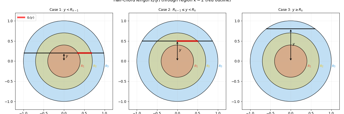
Half-chord length \(\ell_k(y)\) through region \(k = 2\) (red outline) for each of the three cases.

The Two Optical Paths

For a neutron born in region \(i\) targeting region \(j \ge i\), there are two distinct paths along the chord:

1. Same-side path (\(\tau_m\)): gap between the outer boundary of \(i\) and the inner boundary of \(j\):

   (19)\[\tau_m(y) = \sum_{k=i+1}^{j} \tau_k(y)\]

   For adjacent regions \(j = i+1\), this is \(\tau_{i+1}\). For self-collision \(j = i\), \(\tau_m = 0\).

2. Through-centre path (\(\tau_p\)): crosses all inner regions twice (inward to the centre, back out):

   (20)\[\tau_p(y) = \tau_m(y) + 2 \sum_{k=1}^{i} \tau_k(y)\]

Boundary Position Arrays

Cumulative optical distance from the chord midpoint to the outer boundary of region \(k\):

\[x_k(y) = \sum_{m=1}^{k} \tau_m(y), \quad x_0 = 0\]

In code (CPMesh._compute_radial_rcp(), and identically in all three derivation scripts):

bnd_pos = np.zeros((N + 1, n_y))
for k in range(N):
    bnd_pos[k + 1, :] = bnd_pos[k, :] + tau[k, :]

The gaps: gap_d = bnd_pos[j] - bnd_pos[i+1] (same-side) and gap_c = bnd_pos[i] + bnd_pos[j] (through-centre).

Slab Geometry: The \(E_3\) Kernel

The 1D slab half-cell extends from the reflective centre (\(x = 0\)) to the cell edge (\(x = L\)). Geometry built via pwr_slab_half_cell() with coord = CoordSystem.CARTESIAN.

import numpy as np
import matplotlib.pyplot as plt
import matplotlib.patches as mpatches

regions = [
    ('Fuel', 0.9, '#e74c3c'),
    ('Clad', 0.2, '#95a5a6'),
    ('Cool', 0.7, '#3498db'),
]

fig, ax = plt.subplots(figsize=(10, 2.5))
x = 0
for name, width, color in regions:
    rect = mpatches.FancyBboxPatch(
        (x, 0), width, 1, boxstyle="square,pad=0",
        facecolor=color, edgecolor='black', alpha=0.7)
    ax.add_patch(rect)
    ax.text(x + width / 2, 0.5, name, ha='center', va='center',
            fontsize=12, fontweight='bold')
    x += width

ax.set_xlim(-0.1, 2.0)
ax.set_ylim(-0.2, 1.3)
ax.set_xlabel('x (cm)')
ax.set_aspect('equal')
ax.axvline(0, color='red', linestyle='--', linewidth=2,
           label='Reflective BC')
ax.axvline(1.8, color='blue', linestyle='--', linewidth=2,
           label='White BC')
ax.legend(loc='upper right')
ax.set_yticks([])
ax.set_title('Slab Half-Cell Geometry')
plt.tight_layout()

(png)

Slab half-cell: fuel, cladding, and coolant with reflective (left) and white (right) boundary conditions.

Let \(\tau_k = \Sigt{k} \, t_k\) be the optical thickness of region \(k\), and define the cumulative optical path from the cell centre:

\[x_0 = 0, \quad x_{k} = \sum_{m=0}^{k-1} \tau_m\]

The reduced collision probability (unnormalised) is built from two path types:

1. Direct path (same direction along the slab): for \(j > i\),

   (21)\[\delta_d = E_3(g) - E_3(g + \tau_i) - E_3(g + \tau_j) + E_3(g + \tau_i + \tau_j)\]

   where \(g = x_j - x_{i+1}\) is the optical gap between regions.

2. Reflected path (through the reflective centre at \(x = 0\)):

   (22)\[\delta_c = E_3(g_c) - E_3(g_c + \tau_i) - E_3(g_c + \tau_j) + E_3(g_c + \tau_i + \tau_j)\]

   where \(g_c = x_i + x_j\) is the optical path via the centre.

3. Self-collision (\(i = j\)):

   (23)\[r_{ii} = \Sigt{i} t_i - \bigl(E_3(0) - E_3(\tau_i)\bigr)\]

The total reduced CP for \(i \ne j\) is:

\[r_{ij} = \frac{1}{2}(\delta_d + \delta_c)\]

and the within-cell CP is \(P_{ij}^{\text{cell}} = r_{ij} / (\Sigt{i} \, V_i)\), where \(V_i = t_i\) for slab geometry.

Implemented in CPMesh._compute_slab_rcp(). Verified element-by-element against derivations/cp_slab.py::_slab_cp_matrix by test_cp_verification.py::TestDirectPinfComparison::test_slab_pinf_matches_derivation (tolerance \(< 10^{-10}\)).

Concentric Cylindrical Geometry: The Ki₃/Ki₄ Kernel

The Wigner–Seitz cell replaces the square unit cell by a circle of equal area. From area equivalence \(p^2 = \pi R_{\text{cell}}^2\):

(24)\[R_{\text{cell}} = \frac{p}{\sqrt{\pi}}\]

Geometry built via pwr_pin_equivalent() with coord = CoordSystem.CYLINDRICAL.

import numpy as np
import matplotlib.pyplot as plt

fig, ax = plt.subplots(figsize=(6, 6))

regions = [
    (0.9, '#e74c3c', 'Fuel'),
    (1.1, '#95a5a6', 'Clad'),
    (2.03, '#3498db', 'Cool'),
]

for r, color, label in reversed(regions):
    ax.add_patch(plt.Circle((0, 0), r, color=color, alpha=0.5,
                            label=label))
for r, _, _ in regions:
    ax.add_patch(plt.Circle((0, 0), r, fill=False, edgecolor='black',
                            linewidth=1))

y_chord = 0.6
x_max = np.sqrt(regions[-1][0] ** 2 - y_chord ** 2)
ax.plot([-x_max, x_max], [y_chord, y_chord], 'k-', linewidth=2)
ax.annotate('chord at height $y$', xy=(0, y_chord),
            xytext=(0.5, 1.5), fontsize=11,
            arrowprops=dict(arrowstyle='->', color='black'))
ax.plot([0, 0], [0, y_chord], 'k--', alpha=0.5)
ax.text(0.08, y_chord / 2, '$y$', fontsize=12)

ax.set_xlim(-2.5, 2.5)
ax.set_ylim(-2.5, 2.5)
ax.set_aspect('equal')
ax.legend(loc='upper right', fontsize=11)
ax.set_xlabel('x (cm)')
ax.set_ylabel('y (cm)')
ax.set_title('Wigner\u2013Seitz Cell with Chord Integration')
ax.grid(True, alpha=0.3)
plt.tight_layout()

(png)

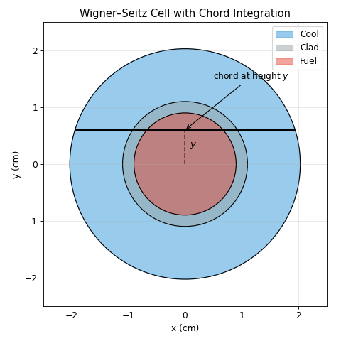
Wigner–Seitz cylindrical cell with concentric annular regions and a chord at height \(y\).

The CP matrix integrates \(\text{Ki}_4\) second-differences over chord heights using composite Gauss–Legendre quadrature (_composite_gauss_legendre()) with breakpoints at each annular boundary to capture chord-length discontinuities.

The CP matrix is computed by integrating the Ki₄ second differences over all chord heights:

(25)\[r_{ij} = 2 \int_0^{R_{\text{cell}}} \bigl[\text{Ki}_4(g) - \text{Ki}_4(g + \tau_i) - \text{Ki}_4(g + \tau_j) + \text{Ki}_4(g + \tau_i + \tau_j)\bigr] \, dy\]

where \(g\) is the optical gap between regions \(i\) and \(j\) along the chord. The factor 2 accounts for the two halves of the chord (by symmetry of the annular geometry, contributions from the left and right halves are equal).

Two path types contribute (same as the slab):

1. Same-side path: source and target on the same side of the chord midpoint.

2. Through-centre path: the neutron crosses the chord midpoint (optical gap \(g_c = x_i + x_j\) from the cumulative boundary positions).

The self-collision term is:

(26)\[r_{ii} = 2\Sigt{i} \int_0^{R_{\text{cell}}} \left[2\ell_i(y) - \frac{2}{\Sigt{i}} \left(\text{Ki}_4(0) - \text{Ki}_4(\tau_i(y))\right)\right] dy\]

The \(y\)-integration is performed with composite Gauss–Legendre quadrature, with breakpoints at each annular boundary to capture the chord-length discontinuities.

Implemented in CPMesh._compute_radial_rcp() with self._kernel = Ki_4. Verified against derivations/cp_cylinder.py::_cylinder_cp_matrix.

Concentric Spherical Geometry: The Exponential Kernel

The spherical cell consists of \(N\) concentric spherical shells. Volumes: \(V_i = \frac{4}{3}\pi(R_i^3 - R_{i-1}^3)\). Surface: \(S = 4\pi R_{\text{cell}}^2\). The kernel is simply \(F(\tau) = e^{-\tau}\) — full 3-D symmetry absorbs all angular variables.

Chord geometry is identical to cylindrical ((18)), but the quadrature weight includes \(y\). For a cylinder (2-D), each chord at height \(y\) represents a line of sources, giving a weight proportional to \(dy\). For a sphere (3-D), each chord represents a ring of sources with circumference \(2\pi y\), giving a weight proportional to \(y\,dy\). In CPMesh._setup_spherical():

# Spherical weight: extra factor of y in the quadrature
self._y_wts = self._y_wts * self._y_pts

Geometry built via mesh1d_from_zones() with coord = CoordSystem.SPHERICAL.

The reduced collision probability has the same structure as cylindrical, but with \(F = \exp(-\cdot)\) and \(y\)-weighted quadrature:

(27)\[r_{ij} = 2 \int_0^{R_{\text{cell}}} \left[e^{-g} - e^{-(g + \tau_i)} - e^{-(g + \tau_j)} + e^{-(g + \tau_i + \tau_j)}\right] y \, dy\]

The self-collision term follows the same pattern:

(28)\[r_{ii} = 2\Sigt{i} \int_0^{R_{\text{cell}}} \left[2\ell_i(y) - \frac{2}{\Sigt{i}} \left(1 - e^{-\tau_i(y)}\right)\right] y \, dy\]

The same code path CPMesh._compute_radial_rcp() handles both cylindrical and spherical, parameterised by kernel and weights. Verified against derivations/cp_sphere.py::_sphere_cp_matrix.

Geometry Comparison

Aspect	Slab	Cylinder	Sphere
Kernel \(F(\tau)\)	\(E_3\) (_e3())	\(\text{Ki}_4\) (_ki4_lookup())	\(e^{-\tau}\)
\(F(0)\)	\(1/2\)	\(\approx 0.4244\)	\(1\)
Quadrature weight	none (scalar)	\(w_i\)	\(w_i \cdot y_i\)
Volume \(V_i\)	\(t_i\)	\(\pi(R_i^2 - R_{i-1}^2)\)	\(\tfrac{4}{3}\pi(R_i^3 - R_{i-1}^3)\)
Angular integration	analytical (in \(E_3\))	numerical (\(y\)-quadrature)	numerical (\(y\)-quadrature)
Surface \(S\)	\(1\)	\(2\pi R_{\text{cell}}\)	\(4\pi R_{\text{cell}}^2\)
Prefactor	1/2 (half-space)	2 (chord halves)	2 (chord halves)
Code path (solver)	CPMesh._compute_slab_rcp()	CPMesh._compute_radial_rcp()	CPMesh._compute_radial_rcp()
Derivation script	derivations/cp_slab.py	derivations/cp_cylinder.py	derivations/cp_sphere.py

The Eigenvalue Problem

Multi-Group Formulation

For \(G\) energy groups, the neutron balance in region \(i\), group \(g\) is:

(29)\[\Sigt{ig} V_i \phi_{ig} = \sum_j P_{ji,g}^{\infty} V_j \left[ \frac{\chi_{jg}}{\keff} \sum_{g'} \nSigf{jg'} \phi_{jg'} + \sum_{g'} \bigl(\Sigs{j,g' \to g} + 2\,\Sigma_{2,j,g' \to g}\bigr) \phi_{jg'} \right]\]

The factor of 2 on \(\Sigma_2\) accounts for both outgoing (n,2n) neutrons (the original neutron is already removed by \(\Sigt{}\)).

Note

Scattering convention. Mixture.SigS[l] uses SigS[g_from, g_to] convention. The in-scatter source uses the transpose: Q_scatter = SigS.T @ phi. This is critical for correct downscatter/upscatter coupling.

Matrix Form

(29) in matrix form: \(\mathbf{A}\Phi = (1/\keff)\mathbf{B}\Phi\) with:

(30)\[A[(i,g),(j,g')] = \delta_{ij}\delta_{gg'}\Sigt{ig} V_i - P_{ji,g}^{\infty} V_j (\Sigs{j,g' \to g} + 2\Sigma_{2,j,g' \to g})\]

(31)\[B[(i,g),(j,g')] = P_{ji,g}^{\infty} V_j \chi_{jg}\, \nSigf{jg'}\]

The analytical verification eigenvalue is \(\lambda_{\max}(\mathbf{A}^{-1}\mathbf{B})\), computed by kinf_from_cp(), which builds the full \(NG \times NG\) matrices and uses numpy.linalg.eigvals. The solver does NOT form these matrices — see Design Decisions.

Power Iteration

Implemented by power_iteration() via the CPSolver protocol:

1. Fission source (CPSolver.compute_fission_source()): \(Q^F_{ig} = \chi_{ig} \sum_{g'} \nSigf{ig'} \phi_{ig'} / \keff\)

2. Fixed-source solve (CPSolver.solve_fixed_source()): \(\phi_{ig}^{\text{new}} = \sum_j P_{ji,g}^{\infty} V_j Q_{jg}^{\text{total}} / (\Sigt{ig} V_i)\)

3. Update \(\keff\) (CPSolver.compute_keff()):

   (32)\[\keff = \frac{\sum_{ig} \nSigf{ig} \phi_{ig} V_i} {\sum_{ig} (\Sigt{ig} - \Sigs{ig}^{\text{out}} - 2\Sigma_{2,ig}^{\text{out}}) \phi_{ig} V_i}\]

   The denominator is the net removal rate: total interactions minus all neutrons that remain in the system (scattered or produced by (n,2n)).

   The (n,2n) subtlety (ERR-015)

   Bug: compute_keff used production/absorption, which is wrong when \(\Sigma_2 \neq 0\) because absorption includes (n,2n) removal but does not credit the two outgoing neutrons. With Sig2[0,0] = 0.01 on region A (2G), the solver converged to \(k = 1.793\) instead of analytical \(k = 2.045\) (12% error).

   First wrong fix: Adding (n,2n) production to the numerator gave \(k = 1.808\) — still wrong because the extra neutron has no fission spectrum \(\chi\) weighting.

   Correct fix: Net-removal denominator (32). When \(\Sigma_2 = 0\), this reduces to \(\nSigf{}\phi V / \Siga{}\phi V\).

   How it hid: All test materials had Sig2 = 0 (zero sparse matrix). The make_mixture API didn’t even accept a sig_2 parameter, making it impossible to construct test materials with nonzero (n,2n).

   Test: test_cp_verification.py::TestN2N::test_n2n_solver_keff_matches_analytical.

   Lesson: When adding a new reaction type, trace it through BOTH the transport solve AND the eigenvalue estimate. Test with the term nonzero.

   For lattice models with reflective (or white) boundary conditions, the leakage term is zero, so this balance is exact.

4. Converge (CPSolver.converged()) when \(|\Delta k| <\) keff_tol and \(\|\Delta\phi\|_\infty <\) flux_tol.

The power iteration algorithm is shared with all ORPHEUS eigenvalue solvers; see The Power Iteration Algorithm in the homogeneous theory for the general formulation.

The power iteration converges to the dominant eigenvalue (\(\keff\)) and the fundamental mode — the unique non-negative eigenvector (Perron–Frobenius theorem) [Hebert2009].

This is implemented in CPSolver, which satisfies the EigenvalueSolver protocol.

Solver Modes: Jacobi and Gauss-Seidel

CPSolver supports two modes via CPParams.solver_mode.

Jacobi (default, CPSolver._solve_fixed_source_jacobi() ). Scattering source from all groups computed simultaneously using the previous iteration’s flux. No inner iterations. One matrix-vector multiply per group per outer.

Gauss-Seidel (CPSolver._solve_fixed_source_gs() ). Groups swept from fast (\(g=0\)) to thermal (\(g=G-1\)). For each group \(g\), inner iterations converge within-group self-scatter before proceeding to \(g+1\).

The inner iteration solves the fixed-point equation:

\[\phi_g = T_g\!\bigl[Q_g^{\text{ext}} + \Sigs{g \to g} \phi_g\bigr]\]

where \(T_g[\cdot]\) is the CP transport operator for group \(g\) (the matrix multiply \(P^T V \cdot / (\Sigt{} V)\)). The operator is exact for a given source, but the source depends on \(\phi_g\) through within-group self-scatter \(\Sigs{g \to g}\).

Why inner iterations matter. The spectral radius of the inner iteration operator is approximately \(\Sigs{g \to g} / \Sigt{g}\). Thermal groups (ratio ~0.6–0.9) need 3–8 inner iterations; fast groups (ratio << 1) converge in 1. Convergence criterion: relative flux change \(\|\phi_g^{(n+1)} - \phi_g^{(n)}\| / \|\phi_g^{(n+1)}\| < \texttt{inner\_tol}\).

Tautological inner residual (ERR-016)

Bug: The original inner convergence check computed \(\|\Sigt{} V \phi_g^{\text{new}} - P^T V Q_g\|\), which is identically zero by construction: \(\phi_g^{\text{new}} \equiv P^T V Q_g / (\Sigt{} V)\), so the check computes \(\|x - x\| = 0\). The inner loop always exited after 1 iteration, making GS functionally identical to sequential-group Jacobi.

How it hid: All 27 eigenvalue tests passed (the outer iteration converged regardless). The n_inner array showed all 1s, interpreted as “fast convergence” rather than “broken check”. A QA review initially concluded that inner iterations are fundamentally unnecessary for CP — this is wrong: the transport is exact for a given source, but the source depends on \(\phi_g\) through self-scatter.

Fix: Changed to relative flux change \(\|\phi^{(n+1)} - \phi^{(n)}\| / \|\phi^{(n+1)}\|\). With the corrected residual, thermal groups genuinely require multiple inner iterations; fast groups converge in 1.

Tests: test_cp_verification.py::TestGSInnerIterations — test_thermal_needs_more_inner_than_fast (thermal > fast inner counts), test_gs_eigenvalue_matches_jacobi (same eigenvalue), test_no_self_scatter_one_inner (zero diagonal in \(\Sigma_s\) converges in 1).

Lesson: A convergence check that compares quantities derived from each other by construction tests nothing. Always verify with a problem that should require multiple iterations.

Convergence diagnostics (stored in CPResult):

Field	Shape	Description
residual_history	(n_outer,)	Neutron balance residual \(\|\Sigt{} V \phi - P^T V Q\|_2\) per outer (both modes)
n_inner	(n_outer, ng)	Inner iteration count per group per outer (GS only; None in Jacobi)

Both modes converge to the same eigenvalue and flux distribution (test_cp_verification.py::TestGSInnerIterations::test_gs_eigenvalue_matches_jacobi).

Solver mode comparison

Jacobi	Gauss-Seidel
All groups from previous flux	Sequential; latest flux from earlier groups
No inner iterations	Inner iterations for within-group self-scatter
Simpler (1 matrix multiply/group/outer)	Faster convergence for strong upscatter

Cross-Section Data Layout

Cross sections flow through two layers:

1. Mixture — per-material: (ng,) arrays for \(\Sigt{}\), \(\Siga{}\), \(\Sigf{}\), \(\nSigf{}\), \(\chi\); (ng, ng) sparse matrices for scattering \(\Sigs{}\) (SigS[0]) and (n,2n) \(\Sigma_2\) (Sig2).

2. CellXS — per-cell on the mesh: (N_cells, ng) arrays mapped from materials by assemble_cell_xs() using mat_ids.

Indexing: xs.sig_t[i, g] is the total macroscopic cross section in spatial cell \(i\) and energy group \(g\). Group 0 = fastest (highest energy); group \(G-1\) = slowest (thermal). Cell 0 = innermost; cell \(N-1\) = outermost.

Scattering convention: SigS[g_from, g_to]. The in-scatter source uses the transpose: Q += SigS.T @ phi (applied per-cell):

for k in range(N):
    mid = self.mat_ids[k]
    Q[k, :] += self._scat_mats[mid].T @ flux_distribution[k, :]
    Q[k, :] += 2.0 * (self._n2n_mats[mid].T @ flux_distribution[k, :])

Verification

106 tests across 6 test files verify the CP implementation against analytical eigenvalues computed independently by the derivation modules.

Consolidated Eigenvalue Solvers (CP-20260405-007)

kinf_from_cp() and kinf_homogeneous() replaced 10 duplicated eigenvalue computations across homogeneous.py, sn.py, moc.py, mc.py, cp_slab.py, cp_cylinder.py, and cp_sphere.py. Both accept optional sig_2 / sig_2_mats for (n,2n) reactions. When omitted, (n,2n) is zero and all previous eigenvalues are preserved.

Eigenvalue Verification Cases

27 core cases: {1, 2, 4} groups × {1, 2, 4} regions × {slab, cylinder, sphere}.

Geometry	Tolerance	Test file	Derivation
Slab (\(E_3\))	\(< 10^{-6}\)	test_cp_slab.py	derivations/cp_slab.py
Cylinder (\(\text{Ki}_4\))	\(< 10^{-5}\)	test_cp_cylinder.py	derivations/cp_cylinder.py
Sphere (\(e^{-\tau}\))	\(< 10^{-5}\)	test_cp_sphere.py	derivations/cp_sphere.py

The cylinder/sphere tolerances are 10x looser because the \(\text{Ki}_4\) table interpolation introduces \(O(\Delta x^2) \approx 6 \times 10^{-6}\) error (see Ki3/Ki4 Table Construction). Confirmed by test_cp_verification.py::TestKi4Resolution.

Additionally, algebraic property tests (test_cp_properties.py) are run for all three coordinate systems:

• Row sums \(= 1\) (neutron conservation)

• Reciprocity: \(\Sigt{i} V_i P_{ij} = \Sigt{j} V_j P_{ji}\)

• Non-negativity: \(P_{ij} \ge 0\)

• Homogeneous limit: 1-region \(P = 1\)

Extended Verification (CP-20260405-005)

31 additional tests in test_cp_verification.py closing 9 QA gaps:

• L0 P_inf comparison (G-1): element-by-element solver vs derivation (tolerance \(< 10^{-10}\))

• Multi-group properties (G-6, W-2): row sums and reciprocity at 2G/4G

• Upscatter (G-2, W-1): eigenvalue with nonzero thermal-to-fast transfer

• (n,2n) (C-2, G-3, W-3): solver \(\keff\) matches analytical with Sig2[0,0] = 0.01

• Optical limits (G-4, G-7): thick (\(\tau \gg 1\), \(P_{ii} > 0.99\)) and thin (\(\tau \ll 1\), high escape)

• Convergence rate (G-5): monotonic error decrease, dominance ratio estimation

• 8-region mesh (G-8): mesh refinement convergence

• GS inner iterations (C-1, G-9): thermal > fast inner counts; no-self-scatter in 1; GS/Jacobi eigenvalue agreement

• Ki4 table resolution (W-6): diminishing returns from 5k to 40k points

Plus 36 diagnostic tests in test_cp_diagnostics.py.

pytest tests/test_cp_slab.py tests/test_cp_cylinder.py \
       tests/test_cp_sphere.py tests/test_cp_properties.py \
       tests/test_cp_verification.py tests/test_cp_diagnostics.py -v

Implementation Details

Why P^T Appears in the Flux Update

With \(P_{ij} = P[\text{birth}_i, \text{collision}_j]\), the neutron balance (4) sums over birth regions (first index of \(P\)), which is a column sum. In matrix form:

\[\Sigt{} V \phi = P^T V Q\]

Hence: \(\phi = P^T V Q / (\Sigt{} V)\).

In code: phi[:, g] = P_inf[:, :, g].T @ source (CPSolver._solve_fixed_source_jacobi()).

Historical bug (ERR-009)

P @ source instead of P.T @ source. Correct for homogeneous problems (\(P\) symmetric) but 8% wrong for the 1G 2-region slab (k=1.373 vs analytical 1.272). Caught by the formal verification suite on the first heterogeneous test case. The bug survived 4 weeks because all prior tests were homogeneous.

Ki₃/Ki₄ Table Construction

_build_ki_tables() (solver) and BickleyTables (derivations) tabulate the functions identically:

1. \(\text{Ki}_3(x_k) = \int_0^{\pi/2} e^{-x_k/\sin\theta} \sin\theta\,d\theta\) at 20,000 points on \([0, 50]\) via scipy.integrate.quad. Boundary value \(\text{Ki}_3(0) = 1\) set analytically.

2. \(\text{Ki}_4\) by cumulative trapezoid from right to left:

   ki4_vals = np.cumsum(ki3[::-1])[::-1] * dx
   

3. Runtime lookup via np.interp (linear interpolation). With \(\Delta x = 0.0025\), error is \(O(\Delta x^2) \approx 6 \times 10^{-6}\).

test_cp_verification.py::TestKi4Resolution confirms that increasing from 5,000 to 40,000 points produces diminishing returns (validating the default 20,000).

Equal-Volume Mesh Subdivision

_subdivide_zone() creates equal-volume cells:

Cartesian: \(x_k = x_0 + k(x_N - x_0)/N\).

Cylindrical. Equal annular volumes: \(V = \pi(R_k^2 - R_{k-1}^2) = \text{const}\). Summing: \(\pi R_k^2 = \pi R_0^2 + k \cdot \pi(R_N^2 - R_0^2)/N\), giving:

\[R_k = \sqrt{R_0^2 + \frac{k}{N}(R_N^2 - R_0^2)}\]

For \(R_0 = 0\): \(R_k = R_N\sqrt{k/N}\).

Spherical. Equal shell volumes: \(V = \frac{4}{3}\pi(R_k^3 - R_{k-1}^3) = \text{const}\), giving:

\[R_k = \left(R_0^3 + \frac{k}{N}(R_N^3 - R_0^3)\right)^{1/3}\]

For \(R_0 = 0\): \(R_k = R_N(k/N)^{1/3}\).

Numerical Evidence: White-BC Approximation Quality

Geometry	CP (white)	SN (reflective)	Difference
Slab 2-region (fuel + mod)	1.272	1.261	+0.9%
Cylinder 2-region (10 cells/zone)	0.995	0.997	-0.2%

The slab shows ~1% overestimation because the white BC smears the anisotropic angular flux at the fuel-moderator interface. The cylindrical discrepancy is smaller because the Wigner–Seitz cell has a larger volume-to-surface ratio, making the boundary angular distribution closer to isotropic. The SN solver uses reflective (specular) BCs; see Boundary Conditions. The ~1% gap between white and reflective BCs is expected physics, not a bug.

Design Decisions

Single CPMesh class (CP-20260404-001). All three geometries share the eigenvalue iteration. Only the kernel construction differs. Adding a geometry requires one _setup_*() method and kernel function, not a new solver class.

Per-group loop (CP-20260404-008). The CP matrix \(P^{\infty}_{ij,g}\) is computed independently per group because \(\tau_{ig} = \Sigt{ig} \ell_i\) varies with group. Vectorising over groups would require restructuring the Ki4 table lookup — deferred as a performance improvement.

Why ORPHEUS does NOT form the full A/B matrices. The analytical verification (kinf_from_cp()) builds the full \(NG \times NG\) matrices and runs numpy.linalg.eigvals. The solver does not, for two reasons:

1. Memory. For 421 groups, 20 cells: \(8420 \times 8420 =\) 567 MB dense. The per-group approach: \(20 \times 20 \times 421 =\) 1.3 MB.

2. Sparsity. The scattering matrix is sparse (downscatter only for fast groups). Per-material sparse storage is far more efficient.

1-group verification is degenerate. \(\keff = \nSigf{}/\Siga{}\) regardless of flux shape. Wrong CP matrices, weight errors, and convention drifts are invisible. The suite tests 1, 2, AND 4 groups.

Note

The 1-group degenerate case masked ERR-001 (z-ordinate weight loss), ERR-002 (scattering transpose), ERR-004 (BiCGSTAB normalisation), ERR-009 (CP transpose), and ERR-015 ((n,2n) keff) — all caught only by multi-group tests. See tests/l0_error_catalog.md.

References

[Carlvik1966]

I. Carlvik, “A method for calculating collision probabilities in general cylindrical geometry and applications to flux distributions and Dancoff factors,” Proc. Third United Nations Int. Conf. Peaceful Uses of Atomic Energy, Vol. 2, 1966.

[Stamm1983] (1,2)

R. Stamm’ler and M.J. Abbate, Methods of Steady-State Reactor Physics in Nuclear Design, Academic Press, 1983.

[Hebert2009] (1,2,3)

A. Hebert, Applied Reactor Physics, Presses internationales Polytechnique, 2009.